Conditions, switching matrix, and path corrections

Path corrections connect transmission paths represented by a DOT graph to the quantities that were actually measured. A frequency-dependent setup must coordinate three steps:

1. select active graph branches;

2. set real instruments and the switching matrix to the frequency;

3. read and apply the correction of the active path.

The DOT reference fully documents nodes, edges, conditions, and the dev/what attributes.

Correction values are commonly supplied through an INI channel and a DAT file. Syntax, units, complex values, and uncertainty are documented in the INI and DAT reference.

Evaluating conditions

EvaluateConditions activates nodes and edges using the explicit context:

mg.EvaluateConditions(context={"frequency": frequency})

With doAction=False, it computes graph state only. This is important for preflight, scan planning, and path validation because those operations must not switch hardware.

An active element may additionally provide an action attribute. Only a direct method call on an object from the context with literal arguments is executed. Arbitrary Python code is not permitted. Actions are suitable for small explicitly configured state changes; prefer the driver for instrument-specific switching logic.

A small matrix may alternatively be switched directly through actions:

SwitchLF [condition="FREQUENCY <= 1e9"
          action="switch.switch_to(0)"]
SwitchHF [condition="FREQUENCY > 1e9"
          action="switch.switch_to(1)"]

mg.EvaluateConditions(context={
    "frequency": frequency,
    "switch": switch_instance,
})

This approach and a frequency-dependent SetFreq implementation in the switch driver are alternatives. Do not set the same relay state through both paths at once.

Switching matrix through SetFreq

A switching matrix is a regular MGraph instrument. Its driver implements SetFreq(frequency) and selects the required relay state from its INI configuration. SetFreq_Devices invokes this method together with the other frequency-dependent instruments:

mg.EvaluateConditions(context={"frequency": frequency})
mg.SetFreq_Devices(frequency)

Conditions and the driver’s switching threshold must use the same range boundaries. For example, the graph selects the LF branch up to and including 1 GHz while the switch driver chooses the same relay state for f <= 1e9.

Before switching, reset a signal generator to a safe initial level or disable RF. This is particularly important when changing frequency activates a different amplifier with a different input limit.

More complex TEM example

digraph {
    Switch [ini="sw_gtem.ini"]
    Sg     [ini="sg.ini"]
    AmpLF  [ini="amp-lf.ini"
            condition="FREQUENCY <= 1e9"]
    AmpHF  [ini="amp-hf.ini"
            condition="FREQUENCY > 1e9"]

    PathSgLF   [ini="sg-lf.ini"]
    PathSgHF   [ini="sg-hf.ini"]
    PathLFCell [ini="lf-cell.ini"]
    PathHFCell [ini="hf-cell.ini"]

    Sg -> SgLF [condition="FREQUENCY <= 1e9"]
    Sg -> SgHF [condition="FREQUENCY > 1e9"]

    SgLF -> AmpInLF [dev=PathSgLF what="S21"]
    SgHF -> AmpInHF [dev=PathSgHF what="S21"]
    AmpInLF -> AmpOutLF [dev=AmpLF what="S21"]
    AmpInHF -> AmpOutHF [dev=AmpHF what="S21"]
    AmpOutLF -> GTEM [dev=PathLFCell what="S21"]
    AmpOutHF -> GTEM [dev=PathHFCell what="S21"]
}

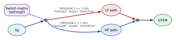
The condition context selects the red or blue correction path. In parallel, SetFreq_Devices sets the switching matrix and all active instruments to the same frequency.

This simplified example shows the forward path only. A real TEM verification adds branches to forward and reverse power meters, including their coupler and cable corrections.

Reading the total correction

get_path_correction returns the total correction between two measurement positions:

from mpylab.tools.aunits import POWERRATIO

correction = mg.get_path_correction(
    names["sg"],
    names["port"],
    POWERRATIO,
)

Without unit, it returns AMPLITUDERATIO. Converting a complex amplitude ratio to a power ratio uses abs(S21) ** 2. Units and uncertainty are preserved.

get_path_corrections additionally returns the individual correction elements. Its "total" key contains the combined result:

details = mg.get_path_corrections("Sg", "GTEM")
total = details["total"]

This detailed form is useful for diagnostics and reports. Application logic should normally use get_path_correction for the total correction.

Applying a correction

Select the direction explicitly according to the physical calculation:

corrected = mg.apply_path_correction(
    measured,
    correction,
    operation="divide",
    magnitude=True,
    output_unit=VOLT,
)

operation is "multiply" or "divide". magnitude=False preserves phase; magnitude=True produces a real magnitude quantity with uncertainty.

Fast repeated application

When processing many values with the same correction, prepare it once:

prepared = mg.prepare_path_correction(
    correction,
    operation="divide",
    magnitude=True,
    output_unit=VOLT,
)

corrected = [
    mg.apply_path_correction(value, prepared)
    for value in measured_values
]

An exactly known constant correction can then use a fast scaling path. Uncertain and unsupported cases automatically fall back to the complete SCUQ calculation.

Reuse the prepared object only while frequency, active graph path, and underlying calibration data remain unchanged. Read and, where appropriate, prepare the correction again after every EvaluateConditions call or frequency change.

Validation rules

• Evaluate conditions before reading a correction.

• Configure switching matrix and graph with identical range boundaries.

• Test boundary frequencies for missing or duplicate paths.

• Keep corrections as SCUQ quantities.

• State multiplication or division and phase removal explicitly.

• Do not reuse prepared corrections across a graph-state change.