Historical Measurement Guide (English Translation)¶

This page provides a faithful English rendering of the historical German guide for measurements in reverberation chambers.

The original historical German source remains available at: Hinweise zur Durchführung von Messungen in Modenverwirbelungskammern.

General¶

All program routines required for instrument control, acquisition, and data evaluation are integrated into the software. The software was implemented in Python (http://www.python.org/).

The architecture allows additional instrument classes to be integrated at any time when a test setup is expanded. Therefore, each specific measurement task can usually be implemented using a comparatively short measurement script that calls existing framework routines.

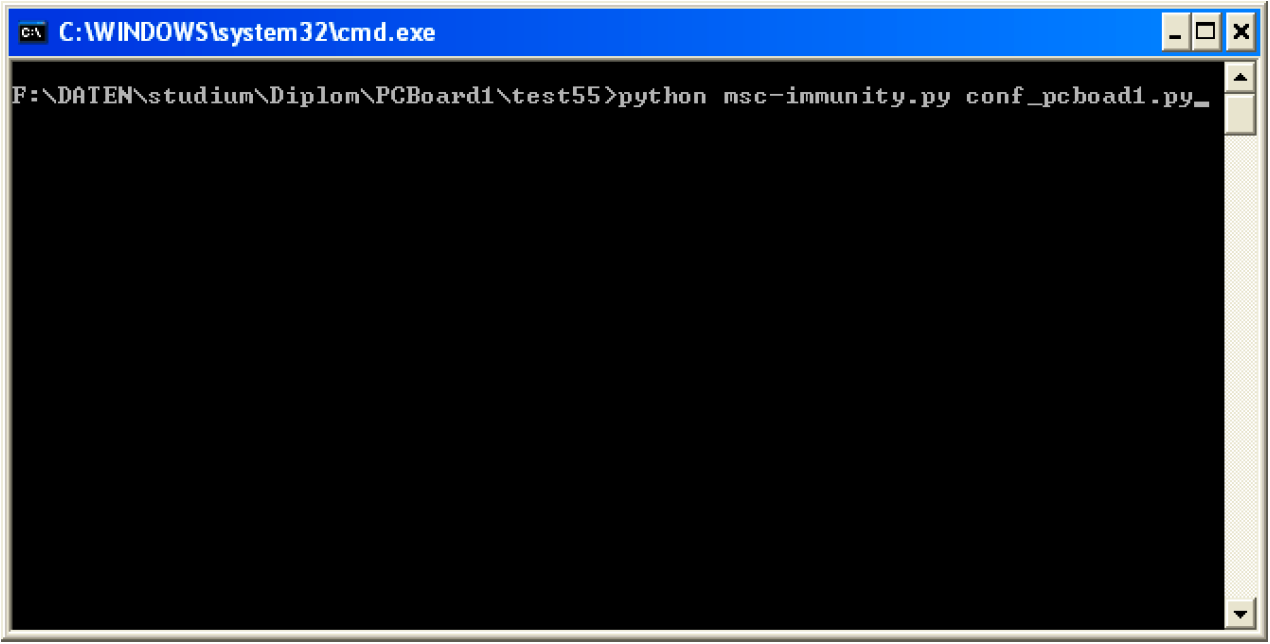
This script is called with a Python configuration file. A historical naming convention used conf_* for such files. The configuration file contains all measurement-relevant parameters, for example:

frequency ranges
step sizes
numbers of tuner positions
evaluation switches and persistence options

For immunity measurements it is recommended, whenever feasible, to include an automated equipment-under-test monitoring mechanism directly in the program flow.

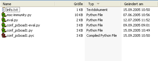
The historical guide also recommends creating one separate folder per measurement campaign. This folder should contain:

the measurement script
the configuration file
optionally a .dot file describing the setup graph

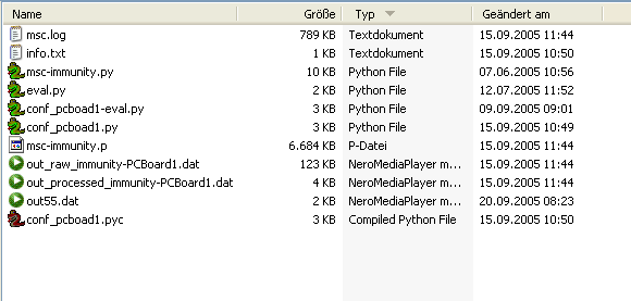
During execution, result files and auxiliary outputs are written into this same folder. If a setup graph is reused across multiple campaigns, the .dot file can also be stored centrally and referenced by path from the configuration file.

Runtime modules, instrument drivers, and generic initialization files do not need to be copied into each campaign folder, because their base paths are configured globally.

A measurement run instantiates MSC in the calling script, either from a fresh state or from existing pickle backup files. The MSC class is responsible for:

communication with instruments
executing measurements
evaluating measurement data
autosave handling
output of raw and processed results

The setup topology (devices and signal paths) is obtained by parsing the .dot file. After each completed stage, the global state can be serialized to pickle and resumed later. This allows pause/resume workflows while keeping full traceability of prior commands and results.

The measurement graph¶

Before running measurements, the physical setup must be defined. The software requires this topology information for correct evaluation of acquired data.

Historically, setup descriptions were written as graphs in .dot files. A representative example from the original guide is shown below.

digraph {
        node [fontsize=12];
        graph [fontsize=12];
        edge [fontsize=10];
        rankdir=LR;

        cbl_sg_amp [ini="M:\\umd-config\\smallMSC\\ini\\cbl_sg_amp.ini" condition="10e6 <= f <= 18e9"] [color=white, fontcolor=white ]
        cbl_amp_ant [ini="M:\\umd-config\\smallMSC\\ini\\cbl_amp_ant.ini" condition="10e6 <= f <= 4.2e9"] [color=white, fontcolor=white ]
        cbl_amp_pm1 [ini="M:\\umd-config\\smallMSC\\ini\\cbl_amp_pm1.ini" condition="10e6 <= f <= 4.2e9"] [color=white, fontcolor=white ]
        sg  [ini="M:\\umd-config\\smallMSC\\ini\\umd-gt-12000A-real.ini"] [style=filled,color=lightgrey]
        amp  [ini="M:\\umd-config\\smallMSC\\ini\\umd-ar-100s1g4-3dB-real-remote.ini" condition="800e6 <= f <= 4.2e9"]
        ant  [ini="M:\\umd-config\\smallMSC\\ini\\umd-rs-HF906_04.ini"] [style=filled,color=lightgrey]
        refant  [ini="M:\\umd-config\\smallMSC\\ini\\umd-rs-HF906_03.ini"] [style=filled,color=lightgrey]
        tuner [ini="M:\\umd-config\\smallMSC\\ini\\umd-sms60-real.ini" ch=1] [style=filled,color=lightgrey]
        pmref [ini="M:\\umd-config\\smallMSC\\ini\\umd-rs-nrvd-2-real.ini" ch=2] [style=filled,color=lightgrey]
        pm1  [ini="M:\\umd-config\\smallMSC\\ini\\umd-rs-nrvd-1-real.ini" ch=1] [style=filled,color=lightgrey]
        pm2  [ini="M:\\umd-config\\smallMSC\\ini\\umd-rs-nrvd-1-real.ini" ch=2] [style=filled,color=lightgrey]
        cbl_ant_pm2 [ini="M:\\umd-config\\smallMSC\\ini\\cbl_ant_pm2.ini" condition="10e6 <= f <= 4.2e9"] [color=white, fontcolor=white ]
        cbl_r_pmr [ini="M:\\umd-config\\smallMSC\\ini\\cbl_r_pmr.ini" condition="10e6 <= f <= 18e9"] [color=white, fontcolor=white ]
        att20 [ini="M:\\umd-config\\smallMSC\\ini\\att20-50W.ini" condition="10e6 <= f <= 18e9"] [color=white, fontcolor=white ]
        a1 [style=filled,color=lightgrey]
        a2 [style=filled,color=lightgrey]

        subgraph cluster_amp {
                label=amp
                amp_in -> amp_out [dev=amp what="S21"]
        }

        sg -> a1 [dev=cbl_sg_amp what="S21"] [label="cbl_sg_amp"]
        a1 -> amp_in
        amp_out -> a2
        a2 -> ant [dev=cbl_amp_ant what="S21"]  [label="cbl_amp_ant"]
        a2 -> pm1 [dev=cbl_amp_pm1 what="S21"]  [label="cbl_amp_pm1"]
        refant -> feedthru [dev=cbl_r_pmr what="S21"]  [label="cbl_r_pmr"]
        feedthru -> pmref [dev=att20 what="S21"]  [label="att20"]
        ant -> pm2 [dev=cbl_ant_pm2 what="S21"]  [label="cbl_ant_pm2"]

        subgraph "cluster_msc" {label=MSC; ant; refant}
        subgraph "cluster_pmoutput" {label="output"; pm1; pm2; pmref;}
}

DOT is used as the graph description language (historical reference: http://www.graphviz.org/).

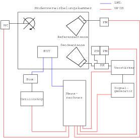
After optional global graph visualization settings, all devices and cable elements are defined as nodes. In the historical example, this includes:

signal generator
several cable elements
attenuator
amplifier
transmit and reference antennas
stirrer (tuner)
power meters

Even cable and attenuation elements were often modeled as graph nodes (instead of only edges) to simplify parameter transfer into the measurement program.

The first attribute block on each node contains measurement-relevant parameters. At minimum, this includes the path to the instrument .ini file. Additional attributes may include operating conditions and actions to execute when conditions become active.

The second attribute block can contain graph-visualization settings.

After node definitions, the actual setup topology is defined by directed edges, which describe how devices are connected and in which signal direction.

The initialization file¶

Each instrument is described by an .ini file. Historically, a file usually contained:

a [description] section
one [Init_Value] section
one or more channel/device-specific sections

Typical fields in [description]:

description (type name)
type (framework class)
vendor
serialnr / deviceid / version data
driver (driver file)

Typical fields in [Init_Value]:

operating frequency range
step sizes
addresses (for example GPIB)
virtual/real flags

Historically, this structure was used both for instruments and for passive path elements such as couplers, attenuators, and cables, each with adapted fields.

Calibration measurements¶

This chapter describes the historical calibration workflow in reverberation chamber operation.

Preparations¶

Before calibration:

ensure instrument availability and addressing
prepare campaign directory and configuration files
prepare the setup graph .dot file
define measurement/evaluation parameter blocks

The dot file¶

For calibration campaigns, the setup graph explicitly describes source path, amplifier path, antenna path, couplers, reference channels, and meter channels.

The graph model must match the real setup topology exactly, because transfer calculations and subsequent immunity evaluations depend on it.

Configuration file¶

The historical calibration configuration contains:

campaign meta settings
tuner settings and sweep ranges
autosave/output control
measurement kernel parameters
references to setup and instrument files

Typical practice was to keep one configuration file per campaign variant and use versioned filenames to preserve reproducibility.

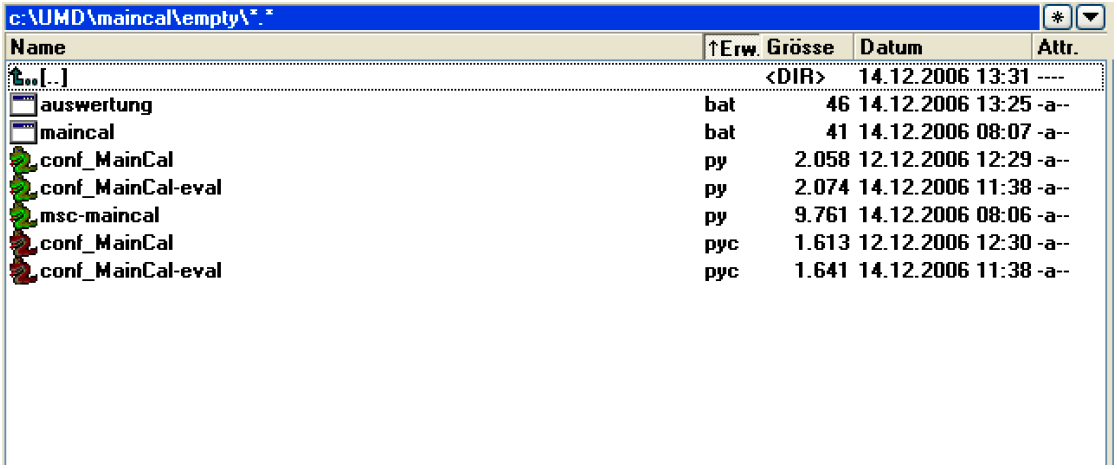
Measurement¶

Calibration measurement execution typically follows:

initialize MSC
load setup graph and configuration
initialize instruments
run calibration sweep(s)
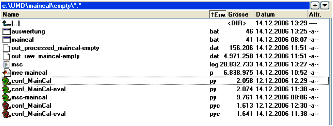
persist raw data and intermediate states
execute evaluation routines
persist processed results

Historical example screenshots:

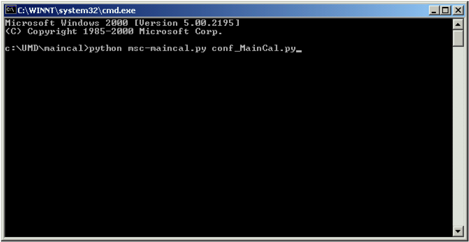
Historical calibration setup view (before run)

Historical calibration setup view (after run)

The measurement program `msc-maincal.py`¶

Historically, msc-maincal.py acted as orchestration script for calibration:

load configuration
create or restore MSC
execute calibration routines
trigger persistence/evaluation

The script is intentionally lightweight and delegates most technical logic to the framework classes and kernels.

Immunity measurements¶

This chapter describes historical workflows for immunity-threshold campaigns.

Measurement sequence¶

Immunity campaigns build on prior calibration data and then run threshold searches over defined frequency and tuner/position spaces.

Historically, a run sequence included:

loading/validating calibration data
selecting immunity target profiles
running controlled source-level adaptation
logging threshold events and operating points
generating processed immunity reports

Preparations¶

Before immunity runs:

verify setup corresponds to calibration topology
verify all references to calibration artifacts
verify fail-safe limits and interlocks
define logging and autosave policies

The dot file¶

The immunity .dot graph remains the topology backbone for signal-path resolution. The same graph model principles apply as in calibration, including device/cable node attributes and edge direction definitions.

Configuration file¶

Immunity configuration historically extended calibration settings with:

threshold logic controls
interruption handling and retry behavior
kernel-specific tuning parameters
output/reporting configuration

Measurement¶

The immunity execution phase typically consists of:

initialize runtime and load persisted context
activate immunity kernel
run threshold search over frequency/position domain
store raw traces and event markers
execute post-processing

Historical run screenshots:

Historical run folder (before immunity run)

Historical run folder (after immunity run)

The measurement kernel `ImmunityThreshholdTDS4.py`¶

The historical immunity kernel controls iterative threshold determination:

set source and setup operating points
read measured response signals
apply threshold criteria
adjust levels/steps according to kernel logic
report threshold hits and status transitions

The historical naming in the source uses Threshhold spelling and is kept unchanged for compatibility.

The measurement program `msc-immunity.py`¶

Historically, msc-immunity.py is the campaign script that orchestrates immunity test execution:

parse campaign configuration
initialize or restore runtime state
invoke immunity kernel with configured ranges
trigger persistence and report generation

As with calibration scripts, orchestration is script-level while technical execution remains in framework classes and kernels.

Graph language references¶

DOT and data-file references used by this historical workflow:

Notes on historical context¶

This translation preserves historical workflow intent and terminology from the legacy document while using current English technical style.

Historical Measurement Guide (English Translation)¶